5 DISCRETE PROBABILITY DISTRIBUTION

Author

Yi Wang

`r`-function	Description
`mean`	Calculate the mean
`sd`, `var`	Calculate the sample standard deviation, use denominator `n-1`. To remove a `NA` value, pass the argument `na.rm=TRUE`.
`weighted.mean(x,wt)`	Calculate a weighted mean (expectation)
`median(x)`	Calculate the median
`rbinom(s,size=n, prob=p)`	Generate `s` random binomial-distributed random values with `n` trials and success probability `p`
`dbinom(x,size=n, prob=p)`	Calculate the density (probability) of a binomial distribution with `x` successes in `n` trials given the success probability `p`
`pbinom(q,size=n, prob=p)`	Calculate the cumulative probability of a binomial distribution less than or equal to `q` successes in `n` trials given the success probability `p`. To calculate the probability greater than `q`, pass an argument `lower.tail=FALSE`.
`hist(x)`	Plot histogram of the 1-D data x: arguments: `main`: main title; `xlab`: x-label; `ylab`: y-label; `col`: color. Pass `freq=FALSE` for a relative frequency histogram.
`rpois(n, lambda)`	Generate `n` random Poisson-distributed values with mean rate of events `lambda`
`dpois(x, lambda)`	Calculate the density (probability) of getting exactly `x` events given a Poisson-distribution with mean rate of events `lambda`
`ppois(x, lambda)`	Calculate the cumulative probability of less than or equal to `x` given a Poisson-distribution with mean rate of events `lambda`

5.1 Probability distribution

5.1.1 Calculate sample mean, standard deviation and variance with equal probability

You can use R to calculate the sample mean, standard deviation, and variance of a given data set using built-in functions like mean(), sd(), and var(). Here’s some sample R code to do that:

Code

# Sample data set
data_set <- c(12, 15, 18, 21, 24, 27, 30, 33, 36, 39)

# Calculate the mean
mean_value <- mean(data_set)
cat("Mean:", mean_value, "\n")

Mean: 25.5

Code

# Calculate the sample standard deviation
std_deviation <- sd(data_set)
cat("Standard Deviation:", std_deviation, "\n")

Standard Deviation: 9.082951

Code

# Calculate the sample variance
variance <- var(data_set)
cat("Variance:", variance, "\n")

Variance: 82.5

Just replace the data_set vector with your actual data, and this code will compute and print the mean, standard deviation, and variance for your data set. Note the results calculated by mean(), sd() and var() assumes each data points occurs with the equal probability 1/n, where n is the number of data points.

5.1.2 Expectation and standard deviation with a given probability distribution

Calculation by definition:

Code

# Define the possible values and their corresponding probabilities
values <- c(1, 2, 3, 4, 5)
probabilities <- c(0.1, 0.2, 0.3, 0.2, 0.2)

# Calculate the mean (expected value)
mean_value <- sum(values * probabilities)

# Print the result
cat("Mean (Expected Value) =", mean_value, "\n")

Mean (Expected Value) = 3.2

Or one can use the following built-in function:

Code

wt <- c(5,  5,  4,  1)/15
x <- c(3.7,3.3,3.5,2.8)
xm <- weighted.mean(x, wt)
xm

[1] 3.453333

To calculate the variance of a probability distribution in R, you can use the following codes.

Code

# Define the values of the random variable (x_i)
values <- c(1, 2, 3, 4, 5)

# Define the probabilities (P(x_i))
probabilities <- c(0.2, 0.3, 0.1, 0.2, 0.2)

# Calculate the mean (expected value) of the random variable
mean_x <- sum(values * probabilities)

# Calculate the variance using the formula
variance <- sum((values - mean_x)^2 * probabilities)

# Print the variance
cat("Variance:", variance, "\n")

Variance: 2.09

5.1.3 Median

Code

# Create a sample vector
data_vector <- c(12, 45, 23, 67, 8, 34, 19)

# Calculate the median
median_value <- median(data_vector)

# Print the median
cat("Median:", median_value, "\n")

Median: 23

5.2 Binomial probability distributions

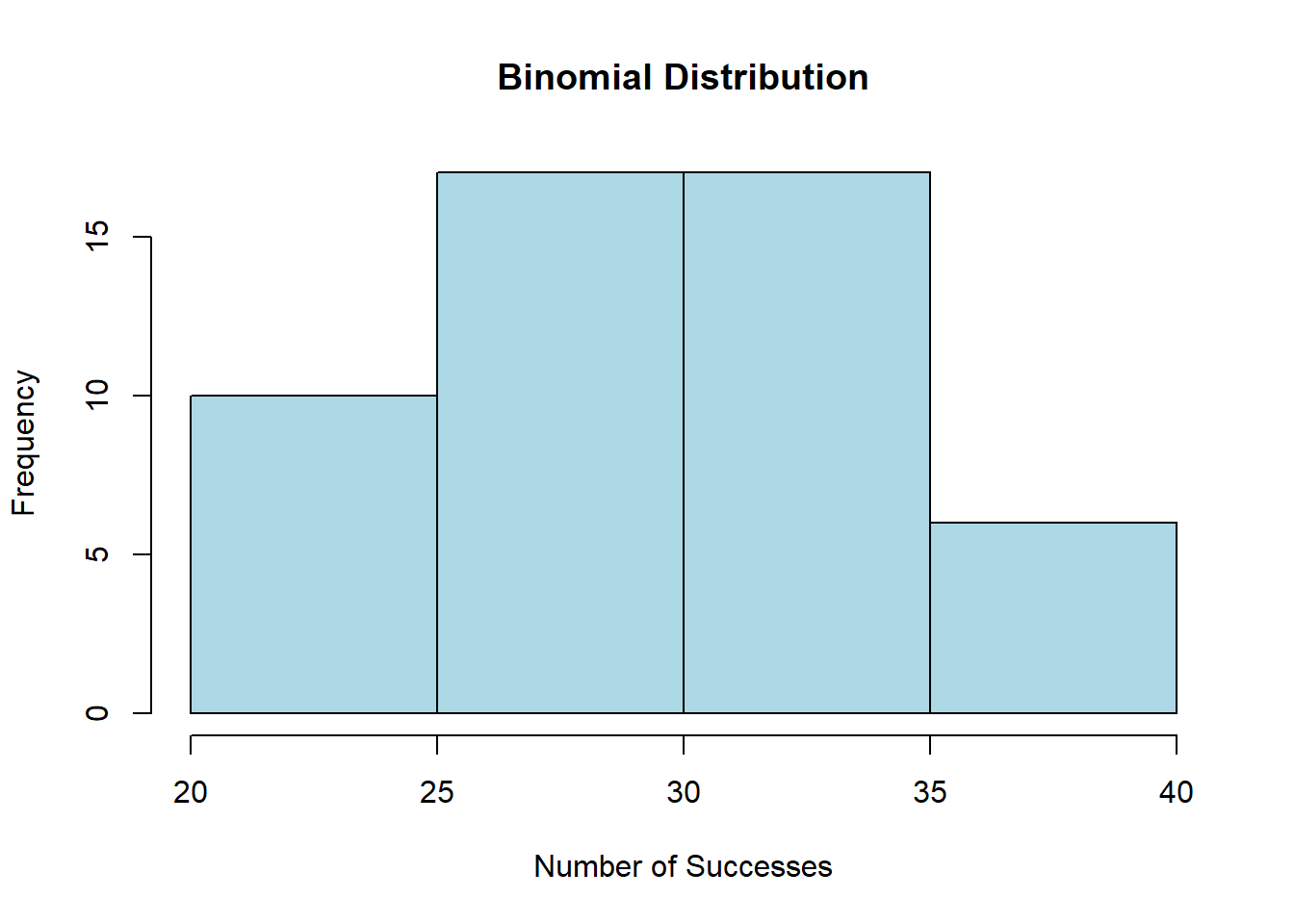
You can generate a data set with a binomial distribution in R using the rbinom() function. This function simulates random numbers following a binomial distribution. Here’s an example code to generate a data set with a binomial distribution:

Code

# Set the parameters for the binomial distribution
n <- 100    # Number of trials
p <- 0.3    # Probability of success in each trial

# Generate a dataset with a binomial distribution
binomial_data <- rbinom(50, size = n, prob = p)

# Print the generated dataset
print(binomial_data)

 [1] 31 39 26 28 20 31 26 28 38 22 27 35 35 37 33 34 40 22 26 22 33 28 24 38 30
[26] 24 37 33 26 32 25 28 29 26 34 31 27 25 35 29 33 32 24 33 30 25 29 32 26 33

Code

# Create a histogram to visualize the data
hist(binomial_data, main = "Binomial Distribution", xlab = "Number of Successes", 
     ylab = "Frequency", col = "lightblue", border = "black")

Code

# verify the mean =np, and var=npq
# Sample mean
mean(binomial_data)

[1] 29.82

Code

# Theoretical mean
n*p

[1] 30

Code

# Sample variance 
var(binomial_data)

[1] 24.27306

Code

# Theoretical variance 
n*p*(1-p)

[1] 21

You can calculate the probability of specific outcomes in a binomial distribution in R using the dbinom() function, which calculates the probability mass function (PMF) of the binomial distribution. Here’s how to use it:

Code

# Set the parameters for the binomial distribution
x <- 2     # Number of successes (the outcome you want to calculate the 
           # probability for)
n <- 10    # Number of trials
p <- 0.3   # Probability of success in each trial

# Calculate the probability of getting 'x' successes in 'n' trials
probability <- dbinom(x, size = n, prob = p)

# Print the calculated probability
cat("Probability of", x, "successes in", n, "trials:", probability, "\n")

Probability of 2 successes in 10 trials: 0.2334744

The pbinom() function in R is used to calculate cumulative probabilities for a binomial distribution. Specifically, it calculates the cumulative probability that a random variable following a binomial distribution is less than or equal to a specified value. In other words, it gives you the cumulative distribution function (CDF) for a binomial distribution.

Here’s the basic syntax of the pbinom() function:

Code

pbinom(q, size, prob, lower.tail = TRUE)

q: The value for which you want to calculate the cumulative probability.

size: The number of trials or events in the binomial distribution.

prob: The probability of success in each trial.

lower.tail: A logical parameter that determines whether you want the cumulative probability for values less than or equal to q (TRUE) or greater than q (FALSE). By default, it is set to TRUE.

The pbinom() function returns the cumulative probability for the specified value q based on the given parameters.

Here’s an example of how to use pbinom():

Code

# Calculate the cumulative probability that X is less than or equal to 3
cumulative_prob <- pbinom(3, size = 10, prob = 0.3)

# Print the cumulative probability
cat("Cumulative Probability:", cumulative_prob, "\n")

Cumulative Probability: 0.6496107

In this example, we’re calculating the cumulative probability that a random variable following a binomial distribution with parameters size = 10 and prob = 0.3 is less than or equal to 3. The result is stored in the cumulative_prob variable and printed to the console.

You can use the pbinom() function to answer questions like “What is the probability of getting at most 3 successes in 10 trials with a success probability of 0.3?” by specifying the appropriate values for q, size, and prob.

5.3 Poisson probability distributions (Optional)

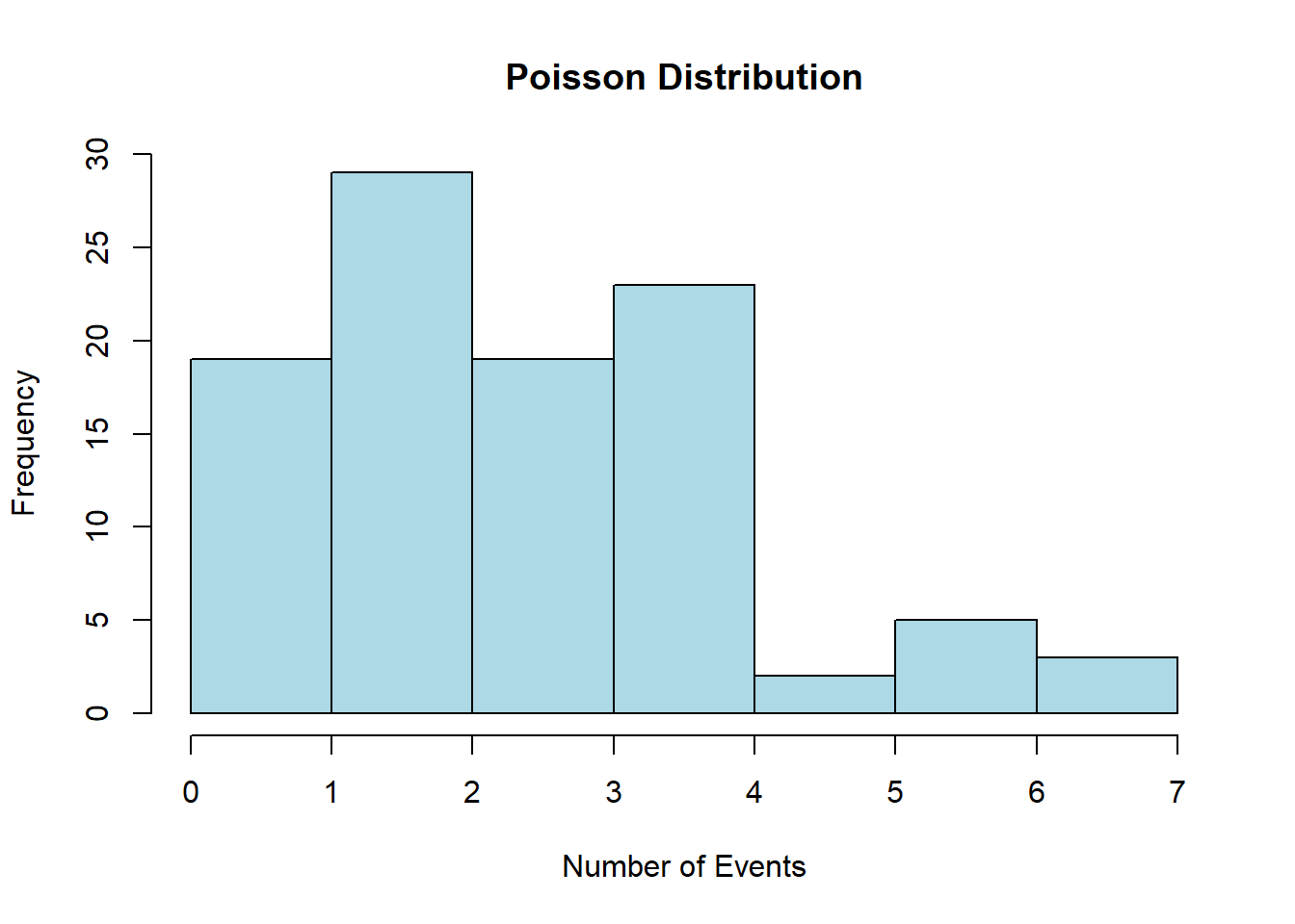
To generate a data set with a Poisson distribution in R, you can use the rpois() function. The Poisson distribution is often used to model the number of events occurring in a fixed interval of time or space when the events happen with a known constant mean rate. Here’s how you can use rpois():

Code

# Set the parameters for the Poisson distribution
lambda <- 3  # Mean (average) rate of events

# Generate a dataset with a Poisson distribution
poisson_data <- rpois(n = 100, lambda = lambda)

# Print the generated dataset
print(poisson_data)

  [1] 3 3 3 4 3 4 3 2 0 2 3 4 2 1 4 3 6 5 4 3 2 2 2 1 4 1 2 0 2 2 1 2 4 2 6 4 0
 [38] 4 3 3 4 1 1 3 7 7 2 6 0 2 3 1 2 5 2 1 2 4 3 4 0 1 1 2 6 4 3 3 2 4 4 7 6 2
 [75] 2 2 2 1 2 1 4 4 2 2 2 3 2 4 3 4 2 2 4 0 4 1 3 4 3 4

Code

# Create a histogram to visualize the data
hist(poisson_data, main = "Poisson Distribution", xlab = "Number of Events", 
     ylab = "Frequency", col = "lightblue", border = "black")

Code

#Theoretical mean = lambda
# Sample mean
mean(poisson_data)

[1] 2.81

Code

#Theoretical variance = lambda
# Sample Variance
var(poisson_data)

[1] 2.579697

To calculate the probability of a specific value occurring in a Poisson distribution in R, you can use the dpois() function. This function calculates the probability mass function (PMF) of the Poisson distribution. Here’s how to use it.

Code

# Set the parameters for the Poisson distribution
x <- 2     # The specific value for which you want to calculate the probability
lambda <- 3  # Mean (average) rate of events

# Calculate the probability of getting exactly 'x' events
probability <- dpois(x, lambda)

# Print the calculated probability
cat("Probability of", x, "events:", probability, "\n")

Probability of 2 events: 0.2240418

To calculate the cumulative distribution function (CDF) for a Poisson distribution in R, you can use the ppois() function. This function calculates the cumulative probability that a Poisson random variable is less than or equal to a specified value. Here’s how to use it:

Code

# Set the parameters for the Poisson distribution
x <- 2  # The specific value to calculate the cumulative probability
lambda <- 3  # Mean (average) rate of events

# Calculate the cumulative probability of getting less than or equal to 'x' events
cumulative_prob <- ppois(x, lambda)

# Print the calculated cumulative probability
cat("Cumulative Probability of less than or equal to", x, "events:", 
    cumulative_prob, "\n")

Cumulative Probability of less than or equal to 2 events: 0.4231901