10 CORRELATION AND REGRESSION

Author

Jieun Park

`r`-function	Description
`data('dataset_name')`	Load a R built-in dataset named by ‘dataset_name’
`names(x)`	Retrieve or set the names of elements in `x`
`attach(df)`	Add a data frame `df` to the search path, which allows you to access the variables within the data frame `df` directly by their names instead of using a normal way such as `df$var`.
`cor(x,y)`	Find the correlation of two vectors `x` and `y`
`qplot(x,y,data)`	Create a quick plot data `(x,y)` in the dataframe `data`
`geom_text(aes(x,y, label))`	Add a `label` at the coordinate `(x,y)` in the current plot.
`lm(y~x, data)`	Perform the linear regression of `y~x`, where `y`,`x` are column names in the dataframe `data`.
`summary(lm_model)`	Summarize the linear model `lm_model` obtained by the R-function `lm`.

10.1 Correlation

We check if a linear correlation exists between two variables using cor() function.

Code

# We can calculate the correlation coefficient between x and y with the 
# following code.
# cor(x, y)

Code

library(tidyverse)
library(patchwork)
data("mtcars")
names(mtcars)

 [1] "mpg"  "cyl"  "disp" "hp"   "drat" "wt"   "qsec" "vs"   "am"   "gear"
[11] "carb"

Code

attach(mtcars)
# positive correlation
qplot(wt, disp, data = mtcars) +
  geom_text(aes(x=2, y=400, label="r = 0.888"))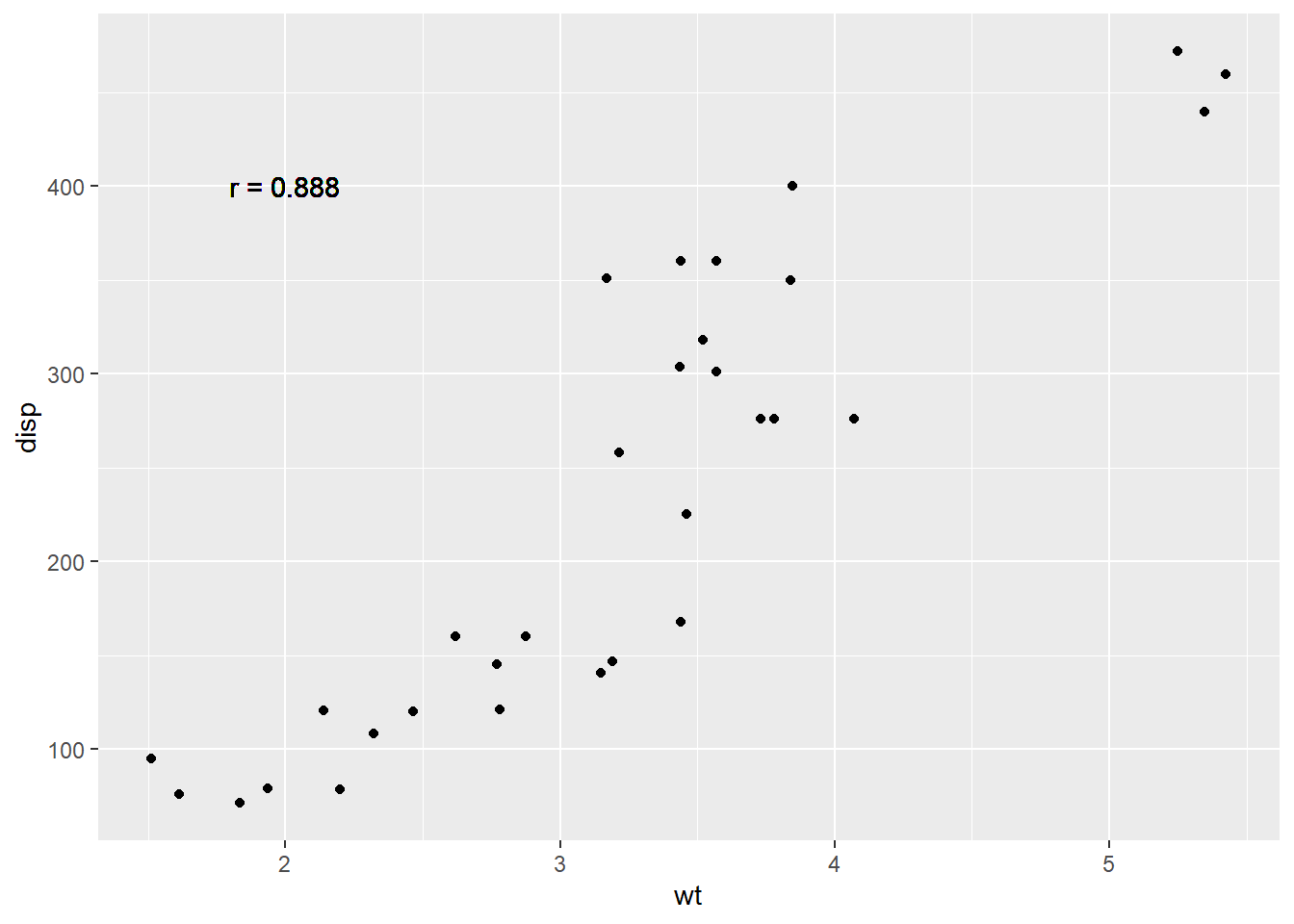

Code

cor(wt, disp)

[1] 0.8879799

Code

# negative correlation
qplot(mpg, wt, data = mtcars)  +
  geom_text(aes(x=30, y=5, label="r = - 0.868"))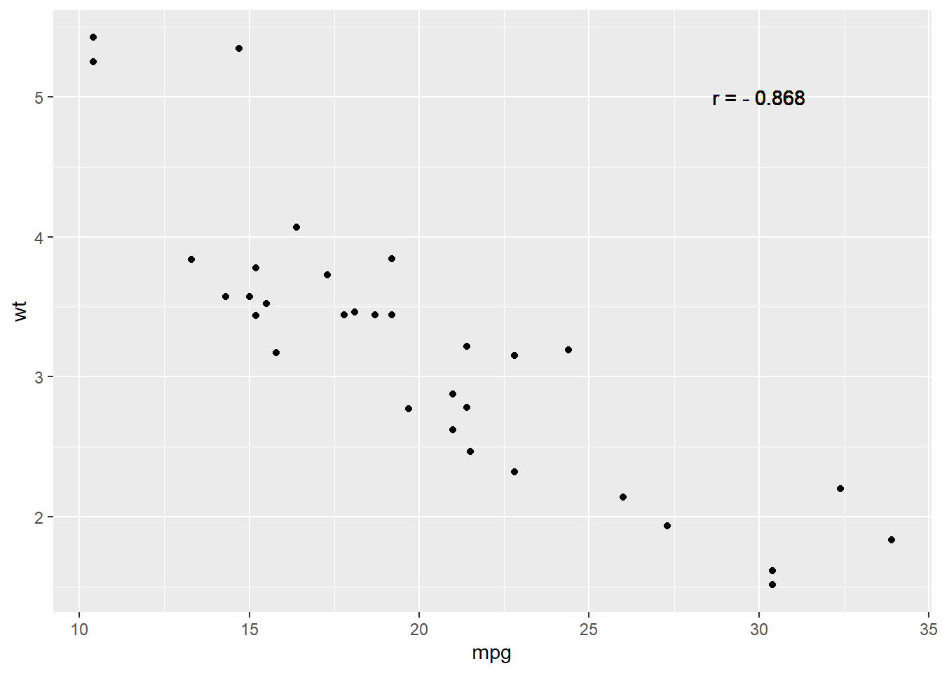

Code

cor(mpg, wt)

[1] -0.8676594

Code

# no correlation
qplot(drat, qsec, data = mtcars)  +
  geom_text(aes(x=4.5, y=22, label="r = 0.091"))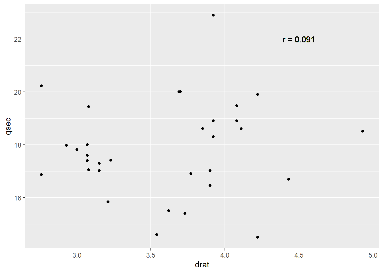

Code

cor(drat, qsec)

[1] 0.09120476

wt and disp have a positive correlation with r =0.888.
wt and disp have a negative correlation with r = -0.868.
wt and disp does not have a significant correlation with r = -0.175.

10.2 Linear regression

Assume we have a data set data with x and y variables and we model their relationship by linear regression. We can find the slope and the intercept of the estimated regression line using the following code.

Code

# res <- lm(y ~ x, data)
# summary(res)

For example, we can find the regression line equation between disp (x-variable, predictor) and wt (y-variable, response) as below.

Code

data("mtcars")
res <- lm(wt ~ disp, mtcars)
summary(res)


Call:
lm(formula = wt ~ disp, data = mtcars)

Residuals:
     Min       1Q   Median       3Q      Max 
-0.89044 -0.29775 -0.00684  0.33428  0.66525 

Coefficients:
             Estimate Std. Error t value Pr(>|t|)    
(Intercept) 1.5998146  0.1729964   9.248 2.74e-10 ***
disp        0.0070103  0.0006629  10.576 1.22e-11 ***
---
Signif. codes:  0 '***' 0.001 '**' 0.01 '*' 0.05 '.' 0.1 ' ' 1

Residual standard error: 0.4574 on 30 degrees of freedom
Multiple R-squared:  0.7885,    Adjusted R-squared:  0.7815 
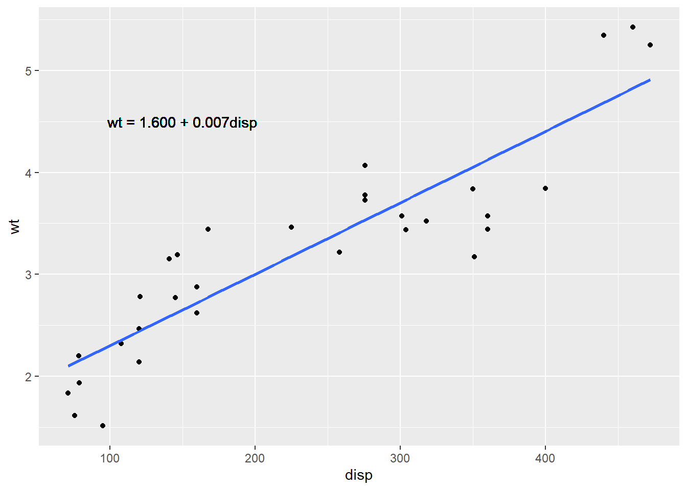
F-statistic: 111.8 on 1 and 30 DF,  p-value: 1.222e-11

The estimated regression line is wt = 1.600 + 0.007 disp since the intercept is 1.6 and the slope is 0.007. Both of them are significantly different from 0 with a significance level \alpha = 0.05 because their p-values are almost 0. The linear relation means that one inch increase in disp (displacement) makes 7 lbs increase in wt (weight). On average, if a car has a one-inch longer displacement, it is 7 pounds heavier.

If a car has 200 inches displacement, then its estimated weight can be calculated as 1.600 + 0.007\cdot200 = 3000 \textrm{ lbs}

We next use the R package ggplot to visualize the data set and the regression line.

Code

ggplot(mtcars, aes(x=disp, y=wt)) +  # define x and y
  geom_point()+                      # scatter  plot
  geom_smooth(method=lm, se=FALSE) + # add a regression line
  geom_text(aes(x = 150, y = 4.5, label = "wt = 1.600 + 0.007disp")) #add a label