Confidence Intervals

https://rafalab.dfci.harvard.edu/dsbook-part-2/inference/estimates-confidence-intervals.html#confidence-intervals

Confidence intervals

  • Confidence intervals are a very useful concept widely employed by data analysts.

  • A version of these that are commonly seen come from the ggplot geometry geom_smooth.

  • Below is an example using a temperature dataset available in R:

Confidence intervals: geom_smooth

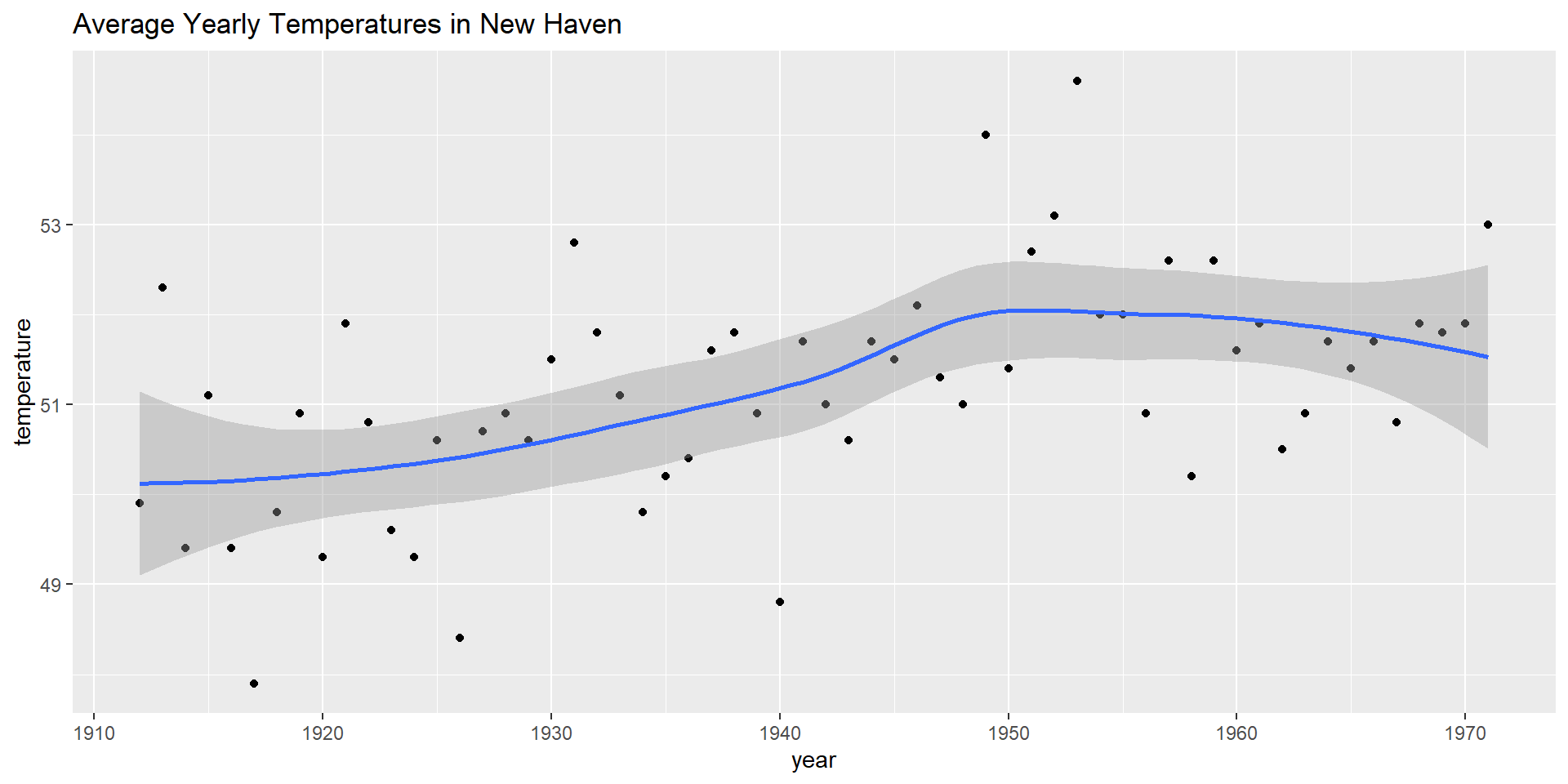
library(tidyverse) #nhtemp is built-in R ts
data.frame(year = as.numeric(time(nhtemp)), temperature = as.numeric(nhtemp)) |> 
  ggplot(aes(year, temperature)) +  
  geom_point() +  # 
  geom_smooth() +  # plot smooth trend-curve (LOESS(small set)/lm (large set)) with a (default) 95% CI
  ggtitle("Average Yearly Temperatures in New Haven") 

Confidence intervals

  • \([0,1]\) is guaranteed to include \(p\), but not useful

  • the spread between -100% and 100%, will be ridiculed for stating the obvious.

  • Even a smaller interval, such as saying the spread between -10 and 10%, will not be considered serious.

  • a very small intervals but misses the mark most of the time will not be considered good

  • We can use the statistical theory to compute the probability of any given interval including \(p\).

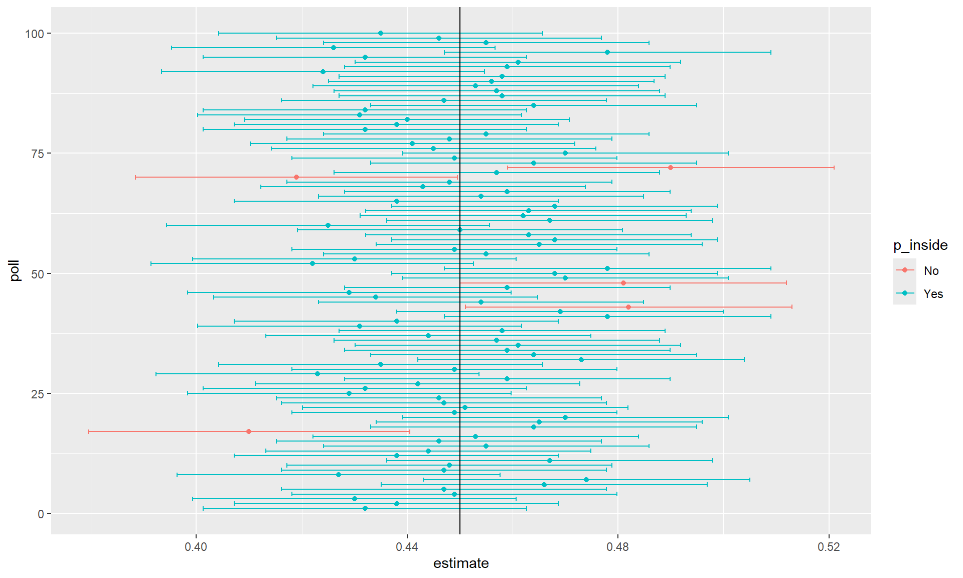
Confidence intervals: MC simulation Parameter

  • To illustrate this we run the Monte Carlo simulation.

  • We use the same parameters as above:

p <- 0.45 
N <- 1000 

Confidence intervals: Simulation

  • And notice that the interval here:
x <- sample(c(0, 1), size = N, replace = TRUE, prob = c(1 - p, p)) 
x_hat <- mean(x) 
se_hat <- sqrt(x_hat*(1 - x_hat)/N) 
c(x_hat - 1.96*se_hat, x_hat + 1.96*se_hat) 
[1] 0.4102262 0.4717738
  • is different from this one:
x <- sample(c(0,1), size = N, replace = TRUE, prob = c(1 - p, p)) 
x_hat <- mean(x) 
se_hat <- sqrt(x_hat*(1 - x_hat)/N) 
c(x_hat - 1.96*se_hat, x_hat + 1.96*se_hat) 
[1] 0.429109 0.490891
  • Keep sampling and creating intervals, and you will see the random variation.

Probability of a Confidence intervals including \(p\)

  • To determine the probability that the interval includes \(p\), we need to compute the following:

\[ \mbox{Pr}\left(\bar{X} - 1.96\hat{\mbox{SE}}(\bar{X}) \leq p \leq \bar{X} + 1.96\hat{\mbox{SE}}(\bar{X})\right) \] Equivalently

\[ \mbox{Pr}\left(-1.96 \leq \frac{\bar{X}- p}{\hat{\mbox{SE}}(\bar{X})} \leq 1.96\right) \]

Confidence intervals with 95% confidence level

  • The term in the middle is an approximately normal random variable with expected value 0 and standard error 1, which we have been denoting with \(Z\), so we have:

\[ \mbox{Pr}\left(-1.96 \leq Z \leq 1.96\right) \]

  • which we can quickly compute using :
pnorm(1.96) - pnorm(-1.96) 
[1] 0.9500042
  • proving that we have a 95% probability.

Confidence intervals of 99% confidence level

  • If we want to have a larger probability, say 99%, we need to multiply by whatever z satisfies the following:

\[ \mbox{Pr}\left(-z \leq Z \leq z\right) = 0.99 \]

  • We use:
z <- qnorm(0.995) 
z 
[1] 2.575829
pnorm(z) - pnorm(-z) 
[1] 0.99

Confidence intervals: significance level \(\alpha\)

  • Confidence interval formulas are given for arbitrary probabilities written as \(1-\alpha\).

  • We can obtain the \(z\) for the equation above using z = qnorm(1 - alpha / 2)

  • for \(\alpha=0.05\), \(1 - \alpha/2 = 0.975\) and we get the \(z=1.96\):

qnorm(0.975) 
[1] 1.959964

A Monte Carlo simulation

  • We can run a Monte Carlo simulation to confirm that, in fact, a 95% confidence interval includes \(p\) 95% of the time.
N <- 1000 
B <- 10000 
inside <- replicate(B, { 
  x <- sample(c(0,1), size = N, replace = TRUE, prob = c(1 - p, p)) 
  x_hat <- mean(x) 
  se_hat <- sqrt(x_hat*(1 - x_hat)/N) 
  between(p, x_hat - 1.96*se_hat, x_hat + 1.96*se_hat) 
}) 
mean(inside) 
[1] 0.9477

A Monte Carlo simulation

  • The following plot shows the first 100 confidence intervals.

set.seed(1) 
tab <- replicate(100, { 
  x <- sample(c(0,1), size = N, replace = TRUE, prob = c(1 - p, p)) 
  x_hat <- mean(x) 
  se_hat <- sqrt(x_hat*(1 - x_hat)/N) 
  hit <- between(p, x_hat - 1.96*se_hat, x_hat + 1.96*se_hat) 
  c(x_hat, x_hat - 1.96*se_hat, x_hat + 1.96*se_hat, hit) 
}) #tab: 4 by 100 matrix
tab <- data.frame(poll = 1:ncol(tab), t(tab)) # add a "poll" index col, t(tab): transpose `tab`
names(tab) <- c("poll", "estimate", "low", "high", "hit") #rename columns
tab <- mutate(tab, p_inside = ifelse(hit, "Yes", "No")) 
ggplot(tab, aes(poll, estimate, ymin = low, ymax = high, col = p_inside)) +  
  geom_point() + 
  geom_errorbar() +  # draw CI from y_min to y_max for each plotted point (poll, estimate)
  # geom_errorbar() does not compute the interval by itself
  coord_flip() +  
  geom_hline(yintercept = p) # draw the true value of p=0.45