Parameters and Estimates

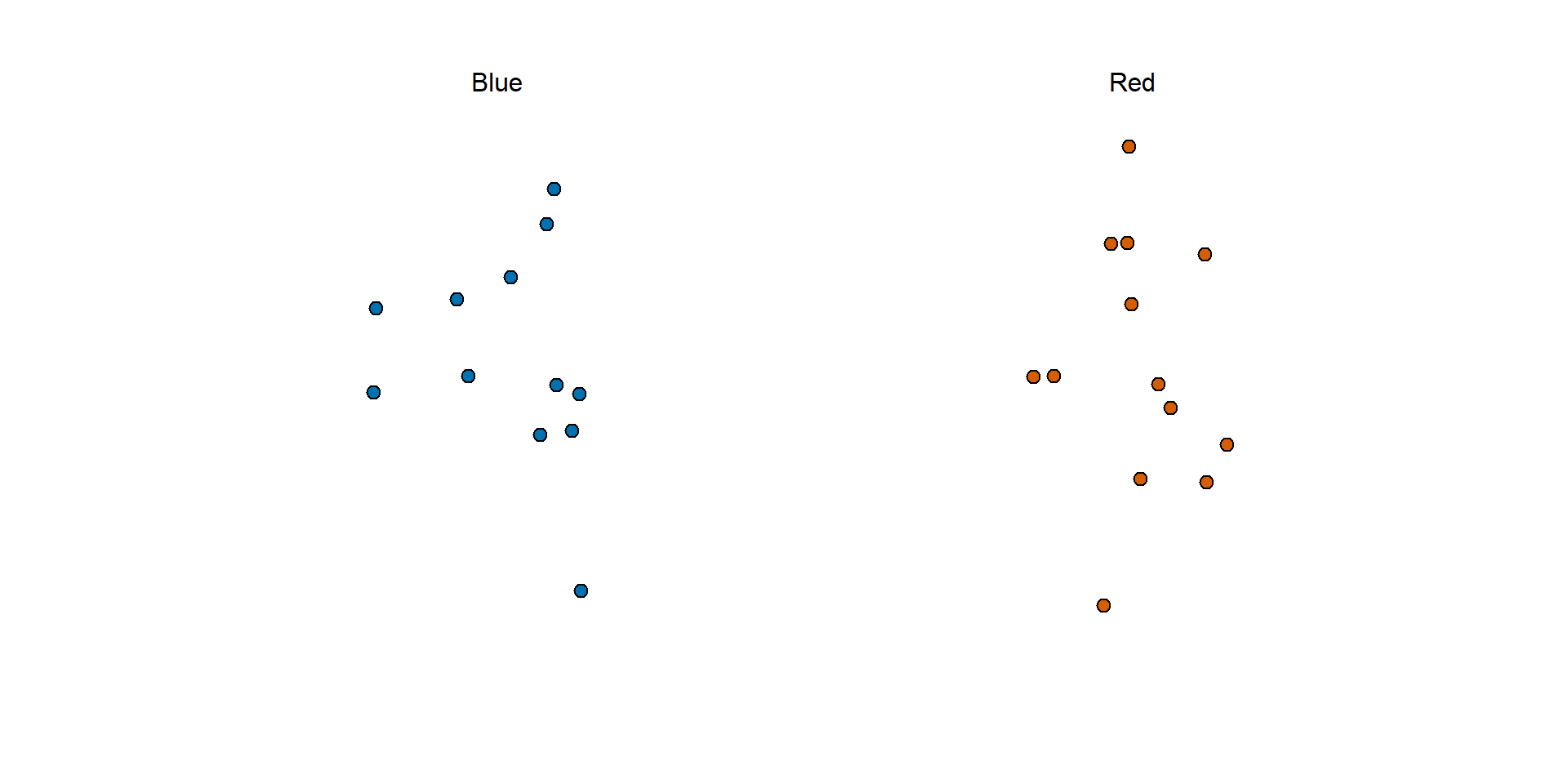
https://rafalab.dfci.harvard.edu/dsbook-part-2/inference/estimates-confidence-intervals.html

The poll example

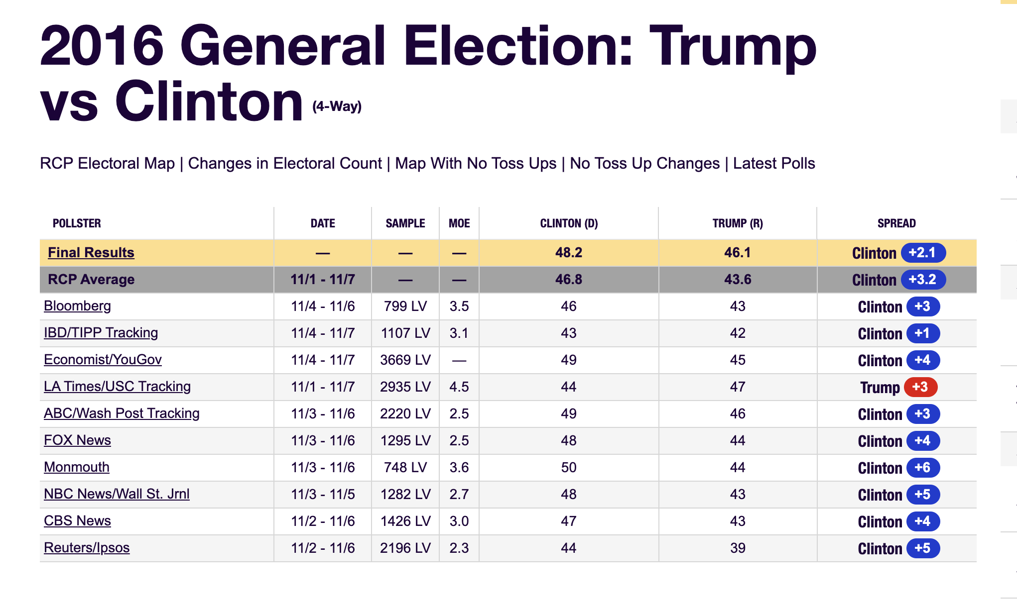
The week before the election Real Clear Politics showed this:

The sampling model for polls

To simulate the challenge pollsters encounter in terms of competing with other pollsters for media attention, we will use an urn filled with beads to represent voters, and pretend we are competing for a $25 dollar prize.
The challenge is to guess the spread between the proportion of blue and red beads in an urn.

The sampling model for polls

Before making a prediction, you can take a sample (with replacement) from the urn.
To reflect the fact that running polls is expensive, it costs you $0.10 for each bead you sample.
Therefore, if your sample size is 250, and you win, you will break even since you would have paid $25 to collect your $25 prize.
Your entry into the competition can be an interval.

If the interval you submit contains the true proportion, you receive half what you paid and proceed to the second phase of the competition.
In the second phase, the entry with the smallest interval is selected as the winner.

set.seed(1)
library(tidyverse) 
library(dslabs) 
take_poll(25) #dslabs function shows a  random draw form thir urn

Populations, samples, parameters, and spread

In statistical class, the beads in the urn are called the population.
The proportion of blue beads in the (unknown) population $p$ is called a parameter.
The 25 beads we see in the previous plot are called a sample.
We want to estimate the spread: $p - (1-p)$ = $2p - 1$.

Goal of Inference

The goal of statistical inference is to predict the population parameter $p$ based on the observed data in the sample.
For example, given that we see 13 red and 12 blue beads, it is unlikely that $p$ > .9 or $p$ < .1.
We want to construct an estimate of $p$ using only the information we observe (the sample).

Example of Samples

The graphs
The code

Observe that in the four random samples shown above, the sample proportions range from 0.44 to 0.60.

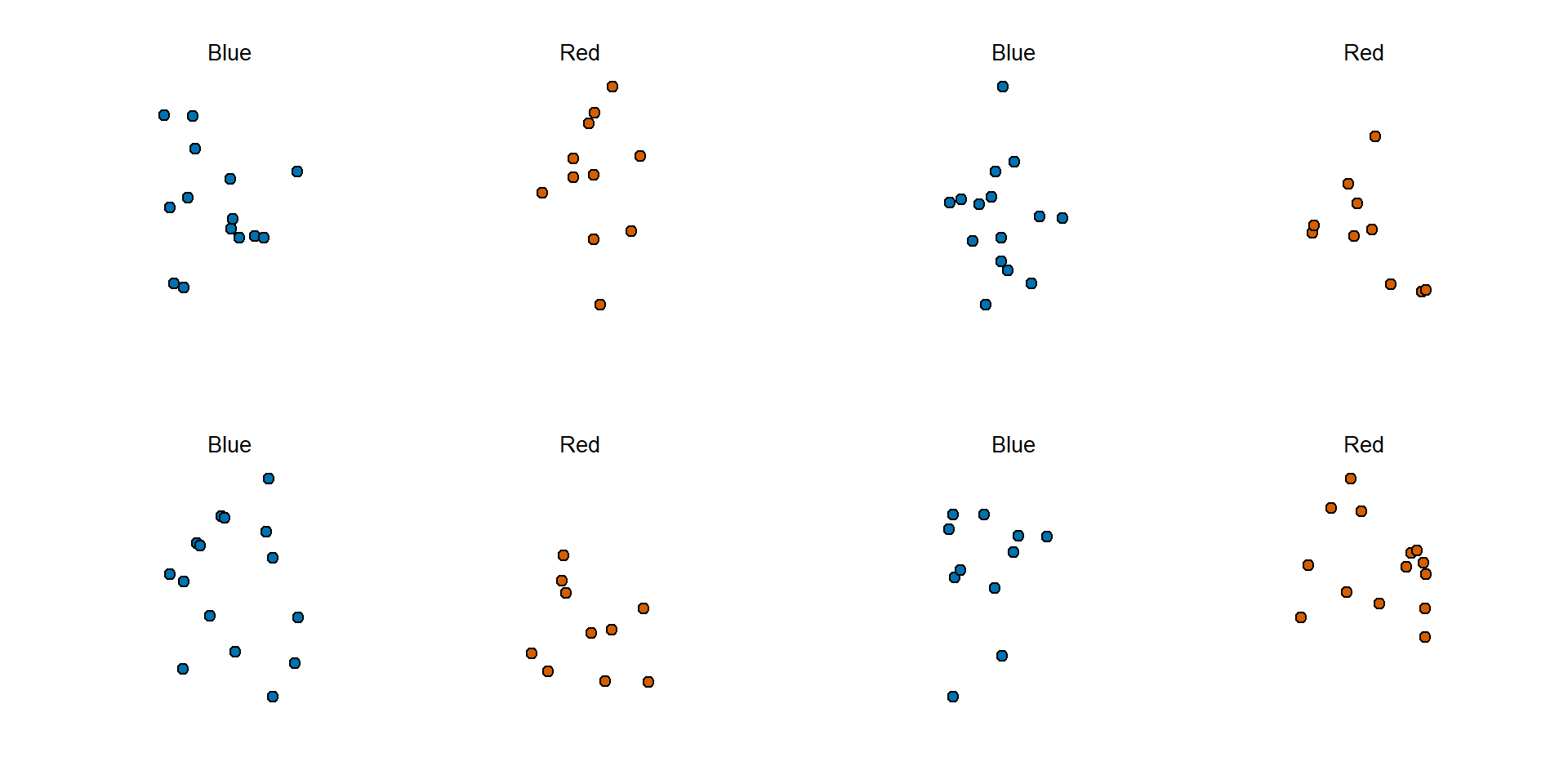
par(mfrow = c(2,2), mar = c(3, 1, 3, 0), mgp = c(1.5, 0.5, 0))  
take_poll(25); take_poll(25); take_poll(25); take_poll(25)

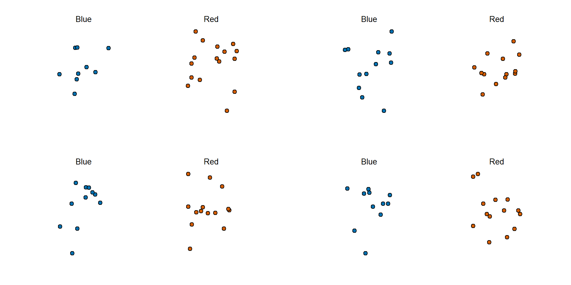
par(): changes plotting layout and margins
mfrow=c(2,2): 2 by 2 grid
mar=c(3,1,3,0): set margins in the order of c(bottom, left, top, right)
mgp=c(1.5, o.5, 0): (postion of the axis title, axis tick labels, axis line)

Parameters

Just as we use variables to define unknowns in systems of equations, in statistical inference, we define parameters to represent unknown parts of our models.
For example, we may want to determine
- the difference in health improvement between patients receiving treatment and a control group,
- investigate the health effects of smoking on a population,
- analyze the differences in racial groups of fatal shootings by police, or
- assess the rate of change in life expectancy in the US during the last 10 years.

Estimating mean by CLT

The properties we learned tell us that:

\[ \mbox{E}(\bar{X}) = p \]

and

\[ \mbox{SE}(\bar{X}) = \sqrt{p(1-p)/N} \]

Properties of our estimate

The law of large numbers tells us that with a large enough poll, $\bar{X}\to p$.
If we take a large enough poll to make our standard error about 1%, we will be quite certain about who will win.
But how large does the poll have to be for the standard error to be this small?
One problem is that we do not know $p$, so we can’t compute the standard error.

SE vs. sample size $n$

The graph
The code

For illustrative purposes, let’s assume that $p=0.51$ and make a plot of the standard error versus the sample size $N$:

p <- 0.51 
N <- 10^seq(1,5, len = 100) # vector of values of N
data.frame(N = N, SE = sqrt(p*(1 - p)/N)) |> ggplot(aes(N, SE)) + geom_line() + scale_x_continuous(breaks = c(10, 100, 1000, 10000), trans = "log10")

Sampple size

The plot shows that we would need a poll of over 10,000 people to achieve a standard error that low.
We rarely see polls of this size due in part to the associated costs.
According to the Real Clear Politics table, sample sizes in opinion polls range from 500-3,500 people.
For a sample size of 1,000 and $p=0.51$, the standard error is:

sqrt(p*(1 - p))/sqrt(1000)

[1] 0.01580823

Distribution of our estimates

The CLT tells us that the distribution function for a sum of draws is approximately normal.
Using the properties we learned: $\bar{X}$ has an approximately normal distribution with expected value $p$ and standard error $\sqrt{p(1-p)/N}$.

What is the probability of within 1% of p?

$$ \[\begin{aligned} \mbox{Pr}(| \bar{X} - p| \leq .01) = \mbox{Pr}(\bar{X}\leq p + .01) - \mbox{Pr}(\bar{X} \leq p - .01) \\ = \mbox{Pr}\left(Z \leq \frac{ \,.01} {\mbox{SE}(\bar{X})} \right) - \mbox{Pr}\left(Z \leq - \frac{ \,.01} {\mbox{SE}(\bar{X})} \right) \end{aligned}\]

Since $p$ is the expected value and $\mbox{SE}(\bar{X}) = \sqrt{p(1-p)/N}$ is the standard error

Estimate the SE

One problem we have is that since we don’t know $p$, we don’t know $\mbox{SE}(\bar{X})$.
using $\bar{X}$ in place of $p$ (CLT)

\[ \hat{\mbox{SE}}(\bar{X})=\sqrt{\bar{X}(1-\bar{X})/N} \]

In our first sample, we had 12 blue and 13 red, so $\bar{X} = 0.48$:

x_hat <- 0.48 
se <- sqrt(x_hat*(1-x_hat)/25) 
se

[1] 0.09991997

Answer to our previous question

pnorm(0.01/se) - pnorm(-0.01/se)

[1] 0.07971926

Therefore, there is a small chance that we will be close.

Margin of error

$1.96$ times the standard error

1.96*se

[1] 0.1958431

Because the probability that we are within 1.96 standard errors from $p$ \[ \begin{aligned} & \mbox{Pr}\left(Z \leq \, 1.96\,\mbox{SE}(\bar{X}) / \mbox{SE}(\bar{X}) \right) - \mbox{Pr}\left(Z \leq - 1.96\, \mbox{SE}(\bar{X}) / \mbox{SE}(\bar{X}) \right) \\ = & \mbox{Pr}\left(Z \leq 1.96 \right) - \mbox{Pr}\left(Z \leq - 1.96\right) = 0.95 \end{aligned} \]

pnorm(1.96) - pnorm(-1.96)

[1] 0.9500042

Central Limit Theorem

There is a 95% probability that $\bar{X}$ will be within $1.96\times \hat{SE}(\bar{X})$, in our case within about 0.2, of $p$.
Observe that 95% is somewhat of an arbitrary choice and sometimes other percentages are used, but it is the most commonly used value to define margin of error.

A Monte Carlo simulation

B <- 10000 
N <- 1000 
x_hat <- replicate(B, { 
  x <- sample(c(0,1), size = N, replace = TRUE, prob = c(1 - p, p)) 
  mean(x) 
})

The problem is, of course, that we don’t know p.

A Monte Carlo simulation

Let’s set p=0.45.
We can then simulate a poll:

p <- 0.45 
N <- 1000 
x <- sample(c(0, 1), size = N, replace = TRUE, prob = c(1 - p, p)) 
x_hat <- mean(x)

In this particular sample, our estimate is x_hat.

B <- 10000 
x_hat <- replicate(B, { 
  x <- sample(c(0, 1), size = N, replace = TRUE, prob = c(1 - p, p)) 
  mean(x) 
})

Simulation results

To review, the theory tells us that $\bar{X}$ is approximately normally distributed, has expected value $p=$ 0.45, and standard error $\sqrt{p(1-p)/N}$ = 0.0157321.
The simulation confirms this:

mean(x_hat)

[1] 0.4500751

sd(x_hat)

[1] 0.01584011

A Monte Carlo simulation: Analysis of x_hat

The graph
The code

A histogram and qqplot confirm that the normal approximation is also accurate:

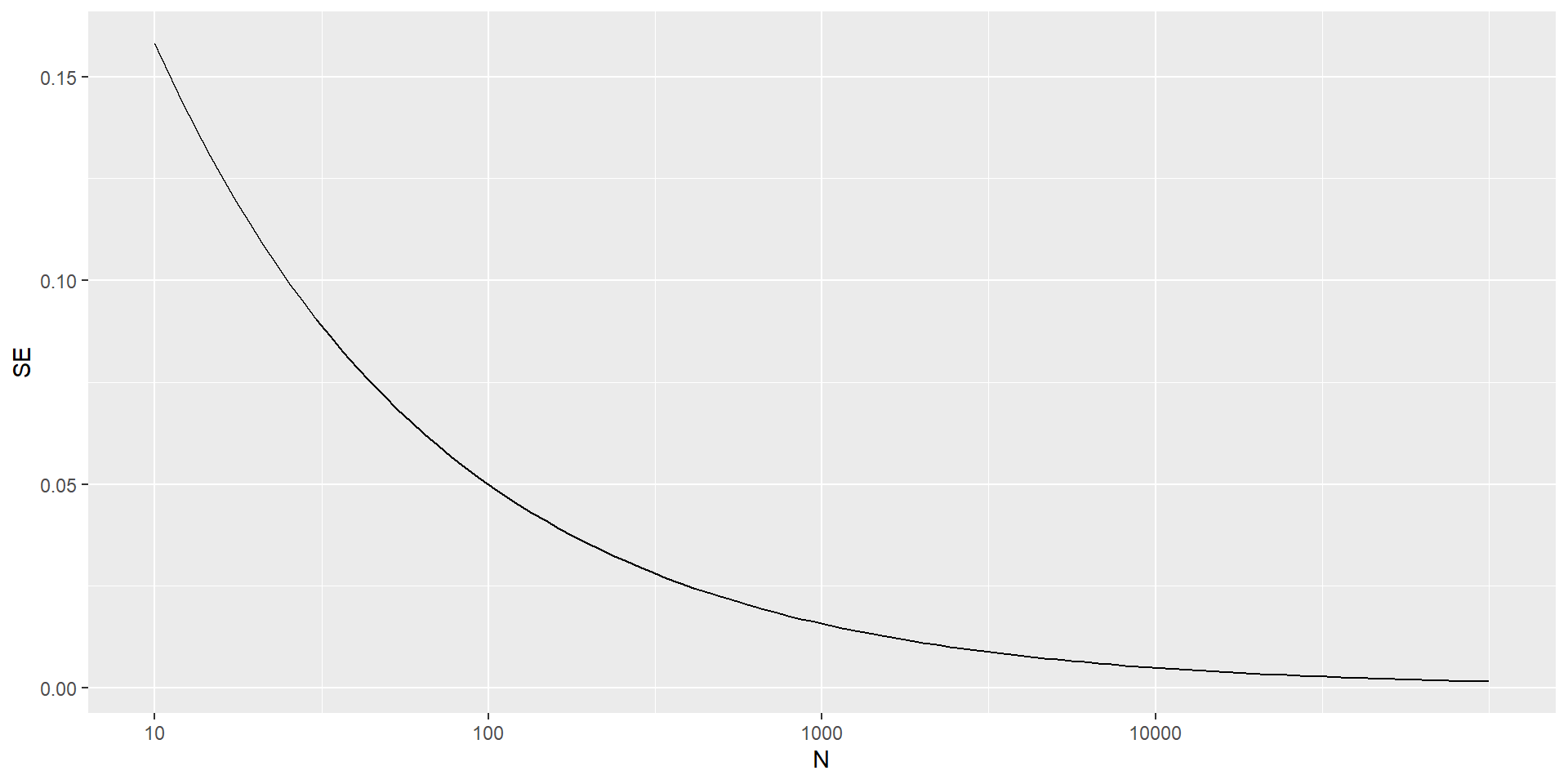
# cache=FALSE: tell Quarto not to cache the reuslts of this chunk

library(tidyverse) 
library(gridExtra) 
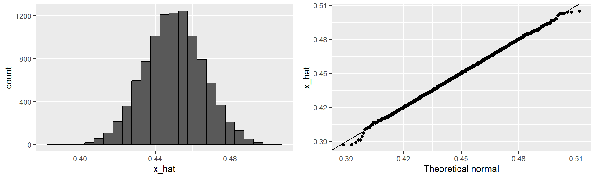
p1 <- data.frame(x_hat = x_hat) |>  
  ggplot(aes(x_hat)) +  
  geom_histogram(binwidth = 0.005, color = "black") #binwidth: refer to the data values 
p2 <-  data.frame(x_hat = x_hat) |>  
  ggplot(aes(sample = x_hat)) +  
  stat_qq(dparams = list(mean = mean(x_hat), sd = sd(x_hat))) + # compare to Normal(mean, sd), not Nornal(0,1)
  geom_abline() +  #geom_abline(intercept=0, slope=1)
  ylab("x_hat") +  
  xlab("Theoretical normal") 
grid.arrange(p1, p2, nrow = 1)

Why not run a very large poll?

For realistic values of $p$, let’s say ranging from 0.35 to 0.65, if we conduct a very large poll with 100,000 people, theory tells us that we would predict the election perfectly, as the largest possible margin of error is around 0.3%.
One reason is that a large poll is expensive.
Another possibly reason is that theory has its limitations.
Polling is much more complicated than simply picking beads from an urn.
Some people might lie to pollsters, and others might not have phones.

Bias: Why not run a very large poll?

However, perhaps the most important way an actual poll differs from an urn model is that we don’t actually know for sure who is in our population and who is not.
How do we know who is going to vote? Are we reaching all possible voters? Hence, even if our margin of error is very small, it might not be exactly right that our expected value is $p$.
We call this bias.
Historically, we observe that polls are indeed biased, although not by a substantial amount.
The typical bias appears to be about 2-3%.

Parameters and Estimates

The poll example

The sampling model for polls

The sampling model for polls

The sampling model for polls

Populations, samples, parameters, and spread

Goal of Inference

Example of Samples

Parameters

Estimating mean by CLT

Properties of our estimate

SE vs. sample size \(n\)

Sampple size

Distribution of our estimates

What is the probability of within 1% of p?

Estimate the SE

Answer to our previous question

Margin of error

Central Limit Theorem

A Monte Carlo simulation

A Monte Carlo simulation

Simulation results

A Monte Carlo simulation: Analysis of x_hat

Why not run a very large poll?

Bias: Why not run a very large poll?