beads <- rep( c("red", "blue"), times = c(2,3))
#rep(x, times=...):repeat each element of x the number of times gieven in times
beads[1] "red" "red" "blue" "blue" "blue"
https://rafalab.dfci.harvard.edu/dsbook-part-2/prob/discrete-probability.html
The term probability is used in everyday language.
Yet answering questions about probability is often hard, if not impossible.
Probability has a very intuitive definition in games of chance.
Probability Theory was born because certain mathematcial computations can give an advantage in games of chance.
Events are fundamental concepts that help us understand and quantify uncertainty in various situations.
An event is defined as a specific outcome or a collection of outcomes from a random experiment.
beads <- rep( c("red", "blue"), times = c(2,3))
#rep(x, times=...):repeat each element of x the number of times gieven in times
beads[1] "red" "red" "blue" "blue" "blue"
For example, if the random experiment is picking 2 beads, we can define events such as first bead is red, second bead is blue, both beads are red, and so on.
In a random experiment such as political poll, where we randomly phone 100 likely voters at random, we can form many million events, for example calling 48 Democrats and 52 Republicans.
We usually use capital letters \(A\), \(B\), \(C\), … to denote events.
If we denote an event as \(A\) then we use the notation \(\mbox{Pr}(A)\) to denote the probability of event \(A\) occurring.
We can combine events in different ways to form new events. For example, if event
\(A\)=first bead is red and second bead is blue, and
\(B\)=first bead is red and second bead is red
then \(A \cup B\) (\(A\) or \(B\)) is the event first bead is red,
while \(A \cap B\) (\(A\) and \(B\)) is the empty event since both can’t happen.
With continuous variables, events will relate to questions, such as Is this person taller than 6 feet?
In these cases, we represent events in a more mathematical form: \(A = \{X > 6\}\).
When we deal the first card, the probability of getting a King is 1/13 since there are thirteen possibilities: Ace, Deuce, Three, \(\dots\), Ten, Jack, Queen, King, and Ace.
If we deal a King for the first card, the probability of a second card being a King decreases because there are only three Kings left: The probability is 3 out of 51.
If you have to guess the color of the first bead, you will predict blue since blue has a 60% chance.
However, if I show you the result of the last four outcomes:
When events are not independent, conditional probabilities are useful.
We use the \(|\) to shorten conditional on. For example:
\[ \mbox{Pr}(\mbox{Card 2 is a king} \mid \mbox{Card 1 is a king}) = 3/51 \]
\[ \mbox{Pr}(A \mid B) = \mbox{Pr}(A) \]
\[ \mbox{Pr}(A \cap B) = \mbox{Pr}(A)\mbox{Pr}(B \mid A) \]
\[ \mbox{Pr}(\mbox{Blackjack in first hand}) = \\ \mbox{Pr}(\mbox{Ace first})\mbox{Pr}(\mbox{Face card second}\mid \mbox{Ace first}) +\\ \mbox{Pr}(\mbox{Face card first})\mbox{Pr}(\mbox{Ace}\mid \mbox{Face card first}) =\\ \frac{1}{13}\frac{16}{51} + \frac{4}{13}\frac{4}{51} \approx 0.0483 \]
\[ \mbox{Pr}(A \cap B \cap C) = \mbox{Pr}(A)\mbox{Pr}(B \mid A)\mbox{Pr}(C \mid A \cap B) \]
\[ \mbox{Pr}(A \cap B \cap C) = \mbox{Pr}(A)\mbox{Pr}(B)\mbox{Pr}(C) \]
Imagine a court case in which the suspect was described as having a mustache and a beard.
The defendant has both and an “expert” testifies that 1/10 men have beards and 1/5 have mustaches.
Using the multiplication rule, he concludes that \(1/10 \times 1/5\) or 0.02 have both.
But this assumes independence!
If the conditional probability of a man having a mustache, conditional on him having a beard, is .95, then the probability is: \(1/10 \times 95/100 = 0.095\)
\[ \mbox{Pr}(B \mid A) = \frac{\mbox{Pr}(A \cap B)}{ \mbox{Pr}(A)} \]
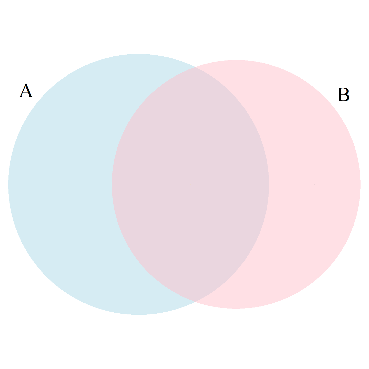
\[ \mbox{Pr}(A \cup B) = \mbox{Pr}(A) + \mbox{Pr}(B) - \mbox{Pr}(A \cap B) \]

library(VennDiagram)
rafalib::mypar() # sets some base plotting parameters, relevant to base R plots
grid.newpage() # clears the curetn grid graphics page
tmp <- draw.pairwise.venn(22, 20, 11, category = c("A", "B"), #(areaA=22, areaB=20, coss.area=11)
lty = rep("blank", 2), # remove the circle borders
fill = c("light blue", "pink"),
alpha = rep(0.5, 2),
cat.dist = rep(0.025, 2), # distance of category lables from the circles
cex = 0, # tex size fore region counts. 0 hides the numbers
cat.cex = rep(2.5,2)) # text size for the category labelsRandom variables are numeric outcomes resulting from random processes (formally, a mapping)
\(X: \text{outcome}\mapsto \mathbb{R}\)
define X to be 1 if a bead is blue and 0 if red:
A more tangible way to think about the probability of an event is as the proportion of times the event occurs when we repeat the experiment an infinite number of times, independently, and under the same conditions.
This is the frequentist way of thinking about probability.
If I have 2 red beads and 3 blue beads inside an urn and I pick one at random, what is the probability of picking a red one? Our intuition tells us that the answer is 2/5 or 40%.
A precise definition can be given by noting that there are five possible outcomes, of which two satisfy the condition necessary for the event pick a red bead.
Since each of the five outcomes has an equal chance of occurring, we conclude that the probability is .4 for red and .6 for blue.
Monte Carlo simulations use computers to perform these experiments.
Random number generators permit us to mimic the process of picking at random.
The sample function in R uses a random number generator:
An example of a probability distribution is:
| Pr(picking a Republican) | = | 0.44 |
| Pr(picking a Democrat) | = | 0.44 |
| Pr(picking an undecided) | = | 0.10 |
| Pr(picking a Green) | = | 0.02 |
For categorical distributions, we can define the probability of a category.
For example, a roll of a die, let’s call it \(X\), can be 1, 2, 3, 4, 5 or 6.
The probability of 4 is defined as:
\[ \mbox{Pr}(X=4) = 1/6 \]
\[ \begin{aligned} F(4) &= & \mbox{Pr}(X\leq 4) \\ &= & \mbox{Pr}(X = 4) + \mbox{Pr}(X = 3) \\ & + & \mbox{Pr}(X = 2) + \mbox{Pr}(X = 1) \end{aligned} \]
When using random number generators you get a different answer each time.
This is fine, but if you want to ensure that results are consistent with each run, you can set R’s random number generation seed to a specific number.
Being able to count combinations and permutations is an important part of performing discrete probability computations.
the function expand.grid
gtools functions: permutatios, combinations.
generate a deck of cards:
suits <- c("Diamonds", "Clubs", "Hearts", "Spades")
numbers <- c("Ace", "Deuce", "Three", "Four", "Five", "Six", "Seven",
"Eight", "Nine", "Ten", "Jack", "Queen", "King")
deck <- expand.grid(number = numbers, suit = suits) # expand.grid makes a df of all combinations of (number, suit). Vary number fist: Ace Diamonds, Deuce Diamonds, ...,
deck <- paste(deck$number, deck$suit) # combine two columns with a space
head(deck,3)[1] "Ace Diamonds" "Deuce Diamonds" "Three Diamonds"
1,2,3:The order matters here: 3,1 is different than 1,3.
(1,1), (2,2), and (3,3) do not appear because once we pick a number, it can’t appear again.
To compute all possible ways we can choose two cards when the order matters, we type, you can use the v option:
What about if the order does not matter? For example, in Blackjack, if you obtain an Ace and a face card in the first draw, it is called a Natural 21, and you win automatically.
If we wanted to compute the probability of this happening, we would enumerate the combinations, not the permutations, since the order does not matter.
When summarizing a list of numeric values, such as heights, it is not useful to construct a distribution that defines a proportion to each possible outcome.
Similarly, for a random variable that can take any value in a continuous set, it impossible to assign a positive probabilities to the infinite number of possible values.
a, gives the proportion of values in the list x that are smaller or equal than a.If I randomly pick one of the male students, what is the chance that he is taller than 70.5 inches?
Since every student has the same chance of being picked, the answer is the proportion of students that are taller than 70.5 inches.
Using the eCDF we obtain an answer by typing:
\[ F(a) = \mbox{Pr}(X \leq a) \]
a and height b is:\[ \mbox{Pr}(a < X \leq b) = F(b)-F(a) \]
Although for continuous distributions the probability of a single value \(\mbox{Pr}(X=x)\) is not defined, there is a theoretical definition that has a similar interpretation.
The probability density function is defined as
\[ F(a) = \mbox{Pr}(X\leq a) = \int_{-\infty}^a f(x)\, dx \]
\[ F(b) - F(a) = \int_a^b f(x)\,dx \]
The intuition is that even for continuous outcomes we can define tiny intervals, that are almost as small as points, that have positive probabilities.
If we think of the size of these intervals as the base of a rectangle, the probability density function \(f\) determines the height of the rectangle so that the summing up of the area of these rectangles approximate the probability \(F(b) - F(a)\).

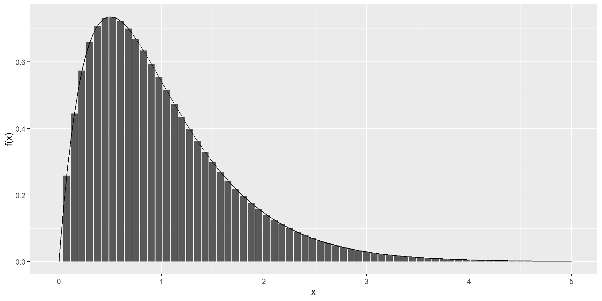
cont <- data.frame(x = seq(0, 5, len = 300), y = dgamma(seq(0, 5, len = 300), 2, 2)) #Gamma(shape=2, rate=2): f(a, b)=b^a/Gamma(a) x^{a-1}e^{-bx}
disc <- data.frame(x = seq(0, 5, 0.075), y = dgamma(seq(0, 5, 0.075), 2, 2))
ggplot(mapping = aes(x, y)) +
geom_col(data = disc) +
geom_line(data = cont) +
ylab("f(x)") \[f(x) = e^{-\frac{1}{2}\left( \frac{x-m}{s} \right)^2} \]
pnorm.m and standard deviation s
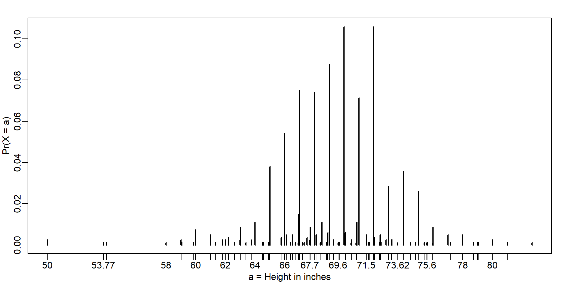
table(): frequency counts. Default drops NA, unless table(x, useNA="ifany")prop.table(): divides those counts by the total count->relative frequencyWhile most students rounded up their heights to the nearest inch, others reported values with more precision.
One student reported his height to be 69.6850393700787, which is 177 centimeters.
The probability assigned to this height is 0.0012315 or 1 in 812.
The probability for 70 inches is much higher at 0.1059113,
Does it really make sense to think of the probability of being exactly 70 inches as being different than 69.6850393700787?
Clearly it is much more useful to treat this outcome as a continuous numeric variable, keeping in mind that very few people, or perhaps none, are exactly 70 inches, and that the reason we get more values at 70 is because people round to the nearest inch.
With continuous distributions, the probability of a singular value is 0.
We therefore could ask, what is the probability that someone is between 69.5 and 70.5?
[1] 0.1031077
[1] 0.1097121
[1] 0.1081743
Although the true height distribution is continuous, the reported heights tend to be more common at discrete values, in this case, due to rounding. We call this situation discretization.
As long as we are aware of how to deal with this reality, the normal approximation can still be a very useful tool.
rnormR provides functions to generate normally distributed outcomes.
Specifically, the rnorm function takes three arguments: size, average (defaults to 0), and standard deviation (defaults to 1), and produces random numbers.
it will permit us to generate data that mimics natural events and answers questions related to what could happen by chance by running Monte Carlo simulations.
If, for example, we pick 800 males at random, what is the distribution of the tallest person? How rare is a seven-footer in a group of 800 males? The following Monte Carlo simulation helps us answer that question:
The normal distribution is not the only useful theoretical distribution.
Other continuous distributions: the student-t, Chi-square, exponential, gamma, beta, and beta-binomial.
R provides functions to compute the density, the quantiles, the cumulative distribution functions and to generate Monte Carlo simulations.
R uses the letters d, q, p, and r in front of a shorthand for the distribution.
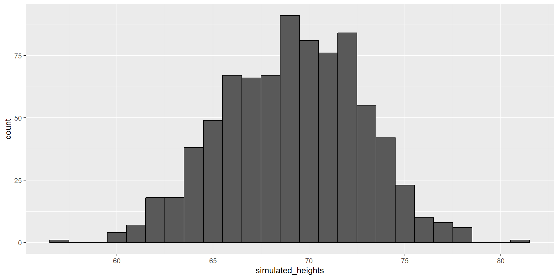
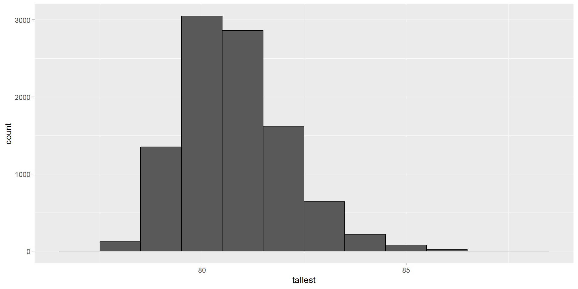
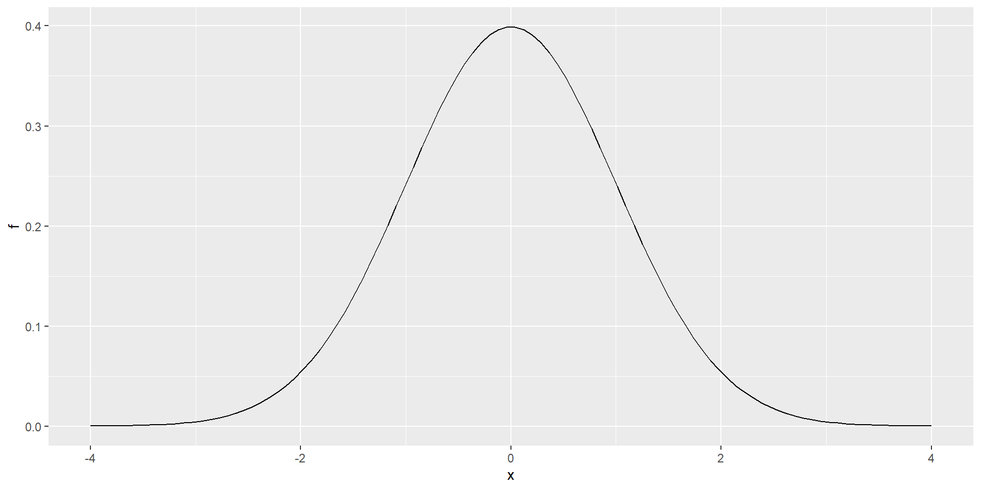
We have already seen the functions dnorm, pnorm, and rnorm for the normal distribution.
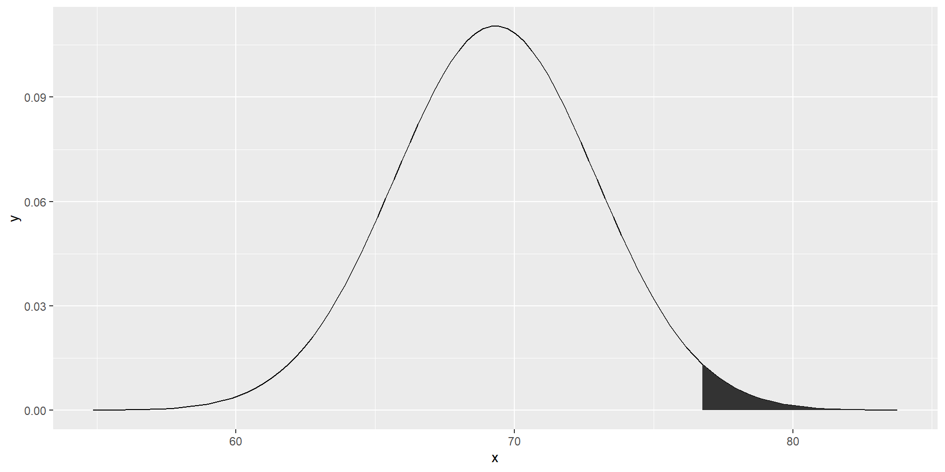
The functions qnorm gives us the quantiles.